Categories
Summarize

VLOOKUP True in Power Query

VLOOKUP True in Power Query

Author: Oz du Soleil

Why Replicate Excel’s VLOOKUP Function?

As much as some people try to avoid VLOOKUP(), it is an incredibly useful function for Excel pros. Those who love it will certainly want to replicate its functionality in Power Query at some point. The thing is, however, depending on which version of VLOOKUP() you need, such as VLOOUP True, it can be quite tricky to implement.

Determining an Exact Match

In truth, we don’t need to do anything special to emulate VLOOKUP’s Exact Match, as this functionality can be replicated by simply merging two tables together.

Making an Approximate Match

Replicating VLOOKUP()’s approximate match is a totally different case than the exact match scenario. It requires some logic to emulate these steps, as we’re not trying to match records against each other. We’re actually trying to find the closest record to our request without going over.

Download the sample file

Explaining VLOOKUP True

It’s always bothered me that VLOOKUP True is considered an approximate match. For example, 64 and 65 could be considered approximate until you need VLOOKUP True to make 65 the line between passing and failing. Suddenly, 64 and 2 have more in common, and 65 is in a whole different world that includes 66, 83 and 99.

This point became relevant recently when I needed to use Power Query to replicate the real function of VLOOKUP True: assigning records to a category or tier.

Up until now, it’s been easy to replicate VLOOKUP-True functionality: just stack up a few conditions, Load To, then move on with life.

Example:

To assign each of these amounts to the categories of Small, Medium or Large, it takes just two conditions.

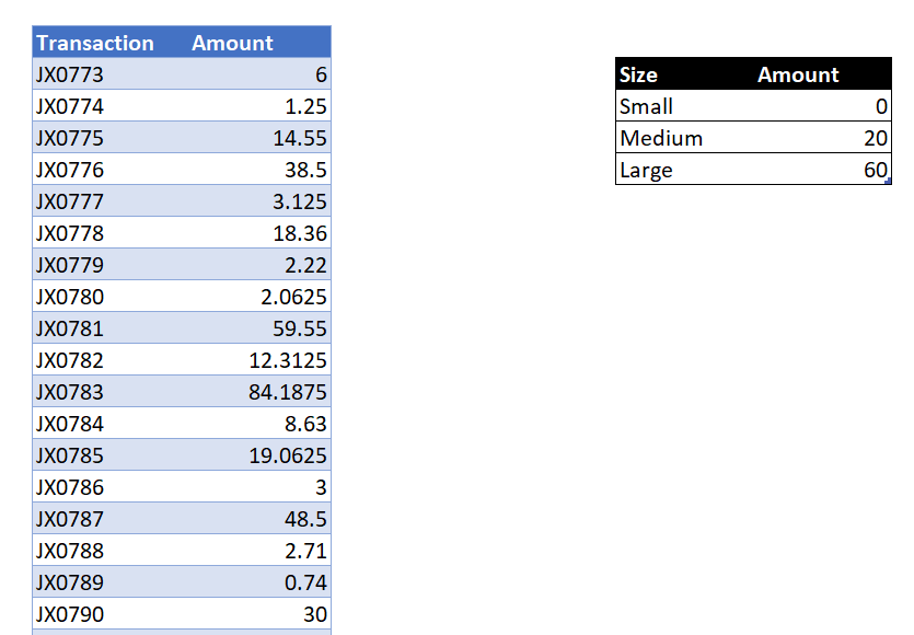
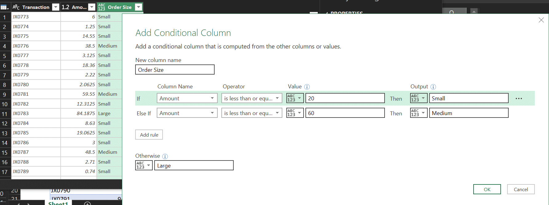
Condition-Stacking… No Way!

Recently, I took on a project where that wouldn’t work because of the way Power Query hardcodes values and does other things that we’ve come to understand are shameful and immoral.

There are two main reasons why this new project was problematic:

  1. Replicating VLOOKUP True with a stack of conditions will hard-code the categories. And unless you’re ready to dig around in the query, you can’t quickly
    • add or remove a tier, or
    • change the size of the tiers.
  2. If you have a lot of tiers to create, that will be a lot of time just stacking up conditions.

Example

Let’s say we need to figure out the right discount amount and make it easy for a user to do something like remove the 30-pound tier and make the 20 – 50 range $2.65.
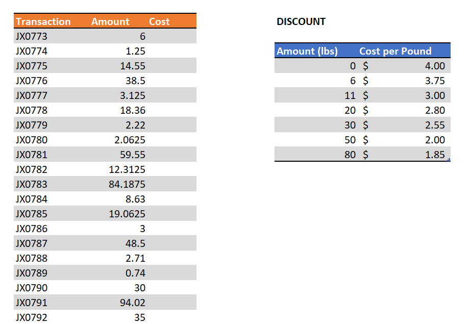
So, how can this be made simpler?

My Solution

After a few hours of internet searches for a solution… I remembered to think TIERS, not about approximate matches. Thus, it would be fantastic if:

  1. I could get the discounts in exactly the right positions between the transactions thus, distinguishing the tier demarcations.
  2. I had a way to identify and delete the tier demarcations when everything is done.

Oh lord, I could suddenly envision the path to glory!

  • Append
  • Sort
  • Fill down
  • Filter

Here’s the video of my solution:

Step 1: Add Column of Flags

My first step was to make a column of flags as an easy visual check during the development process, and an obvious record to delete if everything worked.

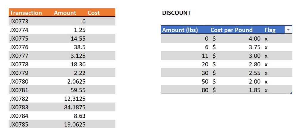
Step 2: Append Queries

With the queries created, the Amount columns needed to be exact so that the queries could be appended. Thus, change the Discounts query’s Amounts (lbs) column to Amounts. Then append the 2 tables:

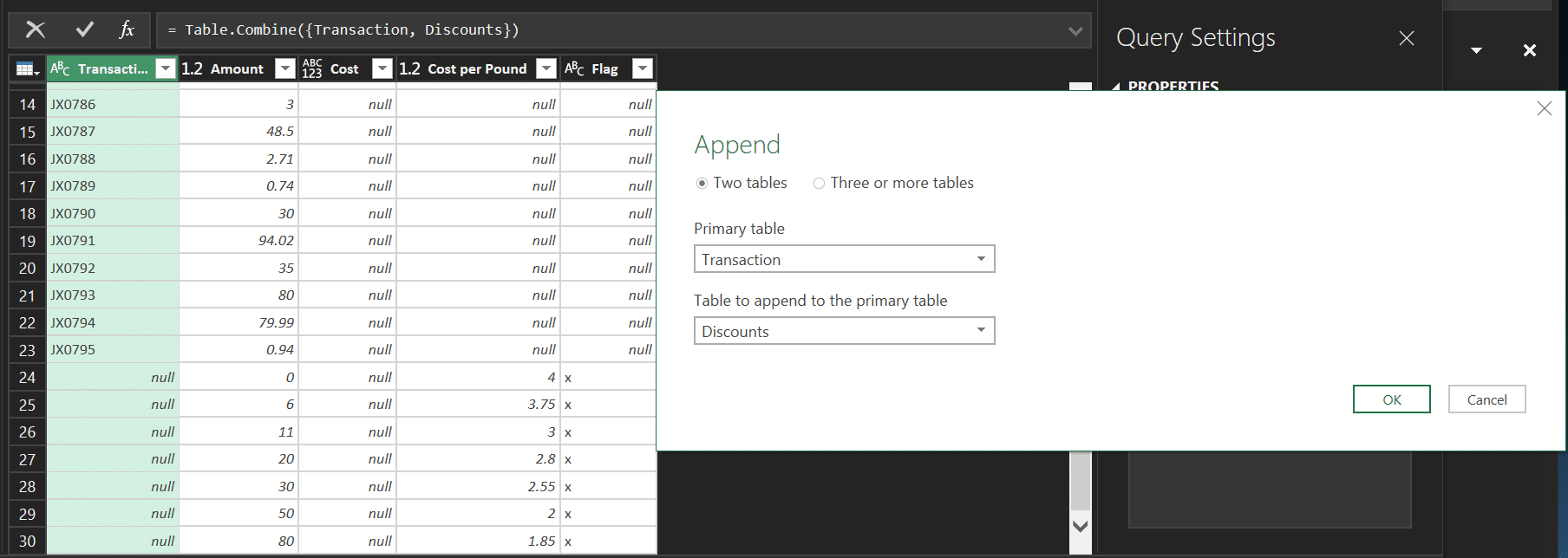
Step 3: Sort by LOOKUP Column

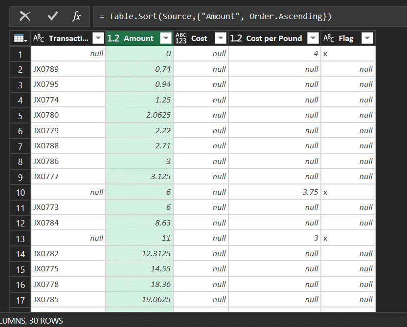
Things were looking great. But here’s the missing step in the video.

After posting it, Szilvia Juhasz noticed that the sort had a problem. The 30 in row 19 is equal to the tier demarcation 30 in row 20, but shows above the demarcation. WRONG! The demarcation needs to be listed first.

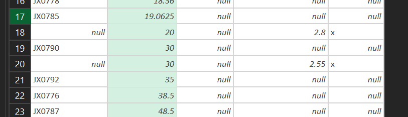
This is solved with a Sort by Transaction to assure that null comes before any transaction where the demarcation is equal to an actual value.

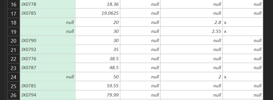
(*NOTE: one thing to think about is tiers that have no values. What happens? Fortunately, that’s not a problem here. The Xs in rows 18 and 19 don’t make problems for us just because there are no orders that are >= 20 and < 30.)

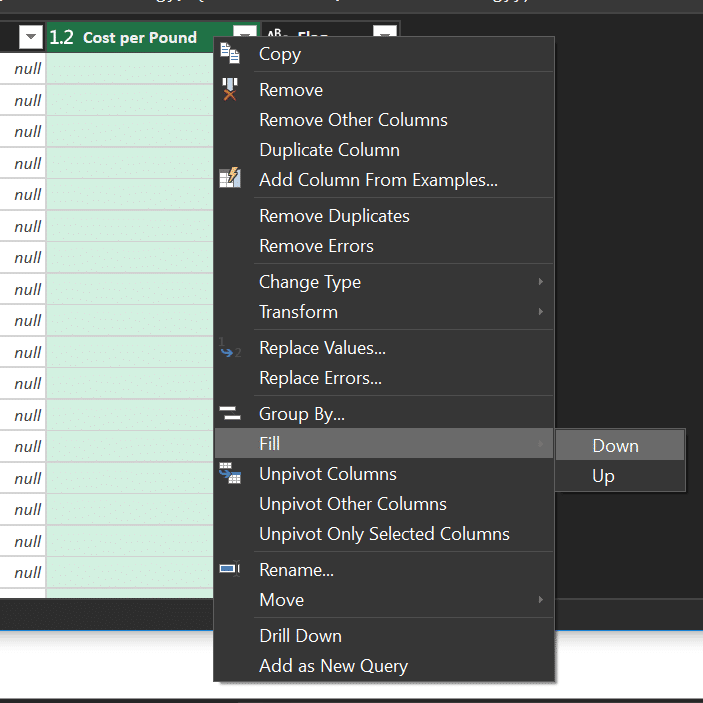
Step 4: Fill Down Column

The Hard Part is Over!

We’ve got this thing whooped now!

In the next screenshot, you can see that the flag isn’t totally necessary. To get rid of the demarcations, we can filter out either, the x in the Flag column or the null in the Transaction column.

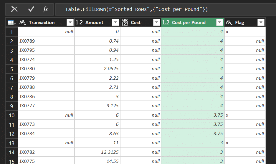
Step 5: Filter out the Placeholder value (X)


Filter out the Xs

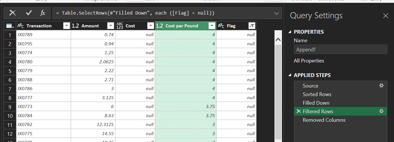
Remove the Flag column then Load To…


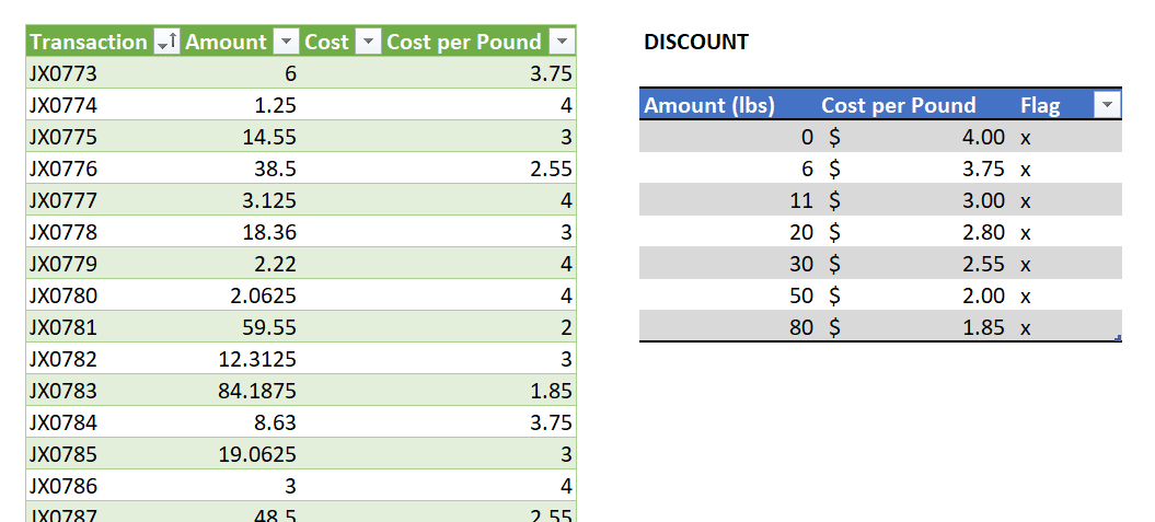
Brothers and sisters, we’re done!! But let’s try it out.

Further Testing

Does it work? With the following changes to the Discounts what happens when we refresh?
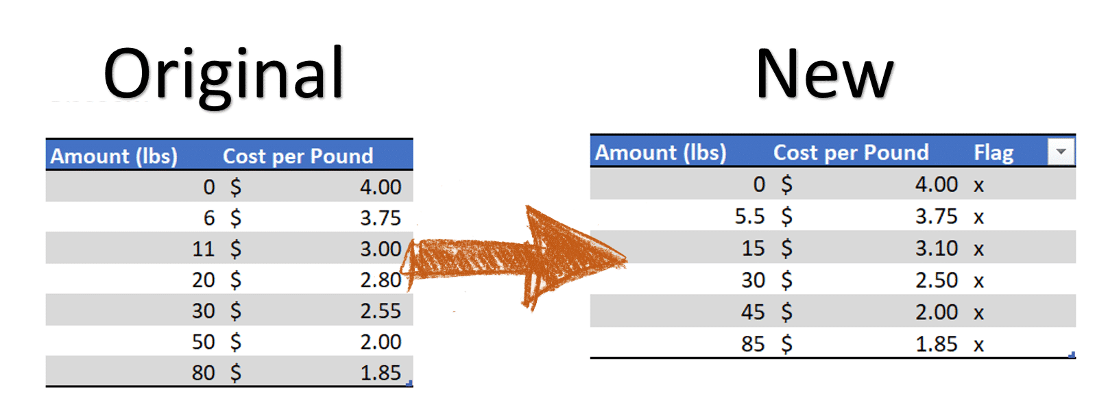
Result!
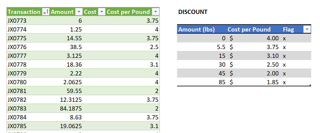
Thanks to Ken Puls and Miguel Escobar for allowing me to share this guest article with you. I appreciate their early efforts and passion for Power Query. So, it’s a real honor to be here with you. Now, go forth and help keep this world’s data clean!

Categories
Summarize

Grouping or Summarizing Data

Grouping or Summarizing Data

Author: Skillwave

The Scenario

One of the most common request of an Excel pro is to group and summarize data. This pattern shows you how to create a compelling report from just a single source of data, which can be refreshed at any time with a single click.

The scenario uses a simple sales table which includes a listing of all products (t-shirts) sold, the date of sale, the sales channel and the total sales dollars for the product on that specific date.

Our Goals

We will start from a source table that has the following columns:

  • Date
  • ProductName
  • ChannelName
  • Amount

Our goal is to create a final report that summarizes that data and lists:

  • The total amount per day for each channel,
  • The total products sold in that channel,
  • All the products sold, and
  • The product with the highest sales.

We can break these into three separate sub-goals:

  1. Create the column that sums all the amounts by date and channel,
  2. Create a new column that represents a list of all the products separated by a commas, and
  3. Create two extra columns that give us the name of the top selling product and its proportion of the total sales.

Let’s find out we can get from the Source Table to the Desired Result.

The Start

Imagine you have a workbook with a worksheet called Sales, where you’ll find a table. Select any cell inside that table, click the Power Query tab and choose From Table.

You’ll now be launched into the Power Query editor.

Goal 1: Grouping and Total Sum Column

Our first step starts by grouping the rows in our table using some criteria. Click the Group By button and set it up using the following criteria:

That should give us a table with a fewer amount of rows because all the data has been grouped by Date and Channel Name. We’ve even managed to create some new data as well, by creating a SUM of the Amount column, and a Count of Distinct Rows (yielding a count of distinct products by channel by day). We’ve also got a list of all products in the final step, which will make a bit more sense later…

A Best Practice: Define DataTypes

Whenever you pull a date into Power Query, we highly recommend that you specifically define the datatype for the date column. If you don’t, the data could be treated as type “any”, which means that it could land as either text or a value in your output instead of a date. It’s not hard to do at all, simply select the column header, go to the Transform tab, and change the Data Type to Date:

So we’ve now got a Total Sales and a Total Products by Channel, finishing our first goal.

Goal 2: Create a Comma Separated List of all Products Sold Each Day

Our next step is to create a formula for a new column that somehow:

  • Takes all the products that were sold on that specific date and channel
  • Creates a list of those products
  • Transforms that List into a table
  • Transposes that table into a table with multiple columns
  • Merges all those columns delimited by a comma

Formula List

This is the formula that does just that using Table.ToList Table.Transpose Table.FromList Table.Column and the Combiner function:

Table.ToList( Table.Transpose(
Table.FromList(
Table.Column([Products], "ProductName")
)
),
Combiner.CombineTextByDelimiter(", ")
)

What this formula is doing?

To better explain what this formula is doing, we are going to do each part of that formula as a new step. The formula defined above basically does all of these steps in a single step.

We start with the most inner function and that is Table.Column([Products], “ProductName”):

What this formula does is simply extract a column from a table and present it to us a List. So we end up having a list with the values from the ProductName column.

The next step is to transform that list into a Table so it can be easier for us to perform other type of operations. The function that transform a list into a table is called Table.FromList and we’ll use it now:
TableToListProductName

As you can see from the picture above, the new column has Table values for that whole column. We did that because we want to use another function to transpose those rows into columns. That function is Table.Transpose and that formula should read like this:

TransposeProductName

The result of that is basically a transposed table. So if we had N amount of rows and only 1 column now we’ll have 1 row with N amount of columns.

Our next step is to combine all the columns using a format similar to “Value1, Value2, Value3, …, ValueN”.

To do that, we use a Table.ToList that automatically does the operation of concatenating all of the strings into a single value. By Default, it uses a comma separator but in this case we want to go with a comma followed by a space (, ) and the second argument of Table.ToList allow us to do so by adding a Combiner function.

In our case, we’ll use this combiner function: Combiner.CombineTextByDelimiter(“, “) that does just exactly what we need.

And once you expand that column by clicking the arrows that go in opposite directions, and once we rename that column, this is the result of it:

RenamedColumn

We created the column that creates the list of all the products that were sold on that day, so we finished our 2nd goal. Let’s go to the next one.

Goal 3: Add columns for top sold Product and participation of it

Our next step is to extract the top product and also its amount on a row by row basis from the column Products which is this case is a table. We can do so by using a new custom column with the following Table.Max function:

Ranking

Once you create this new column, you’ll notice that it’ll populate with records which is a special type of data representation in Power Query and what we need is to extract the ProductName and Amount from that record.

We can do so by simply clicking on the opposite arrows icon that are next to the name of this new column. Click on that icon and you’ll notice a new selection window where you can select what columns you want to extract from that record. For now, just select the ProductName and the Amount columns.

Once we rename those columns this is how our table should look like:

Reportpreview

We are almost there! we are missing the division of the Top Product amount over the Total Sales so we can get a % out of it. Let’s do so by adding a new custom column:

Divide

After spending some more time cleaning the data, this should be the result of our hard work:

Final Result

You can click on Close & Load to save this table to your Workbook or inside your Data Model.

Note that you can refresh this at any time and it’ll work as desired.

Transform it into a Function

There are many ways to transform this into a function, but the basics of creating a function go into making a part of the whole code a variable.

Which one would you choose to make a variable? Let us know in the comments section below

This time, we’re choosing a simple variable. Since we need the Source step to be a table, let’s define that as our variable.

  1. First we go to the View tab and click on Advanced Editor
  2. Then we look at the M code in this Editor and replace the one that we’re trying to make a variable
  3. We replace it with a variable and add the variable before the code as shown in the picture below

Function

Now we need to put this to the test. Let’s create a blank query and grab all the tables from our current Workbook using Excel.CurrentWorkbook():

Excel.CurrentWorkbook

Next we add a custom column by using the name of the function that we just created which is the name of the Query SalesReport and the result should look like this:

ResultFunction