Author: Skillwave
One of the most common request of an Excel pro is to group and summarize data. This pattern shows you how to create a compelling report from just a single source of data, which can be refreshed at any time with a single click.
The scenario uses a simple sales table which includes a listing of all products (t-shirts) sold, the date of sale, the sales channel and the total sales dollars for the product on that specific date.
We will start from a source table that has the following columns:
Our goal is to create a final report that summarizes that data and lists:
We can break these into three separate sub-goals:
Let’s find out we can get from the Source Table to the Desired Result.
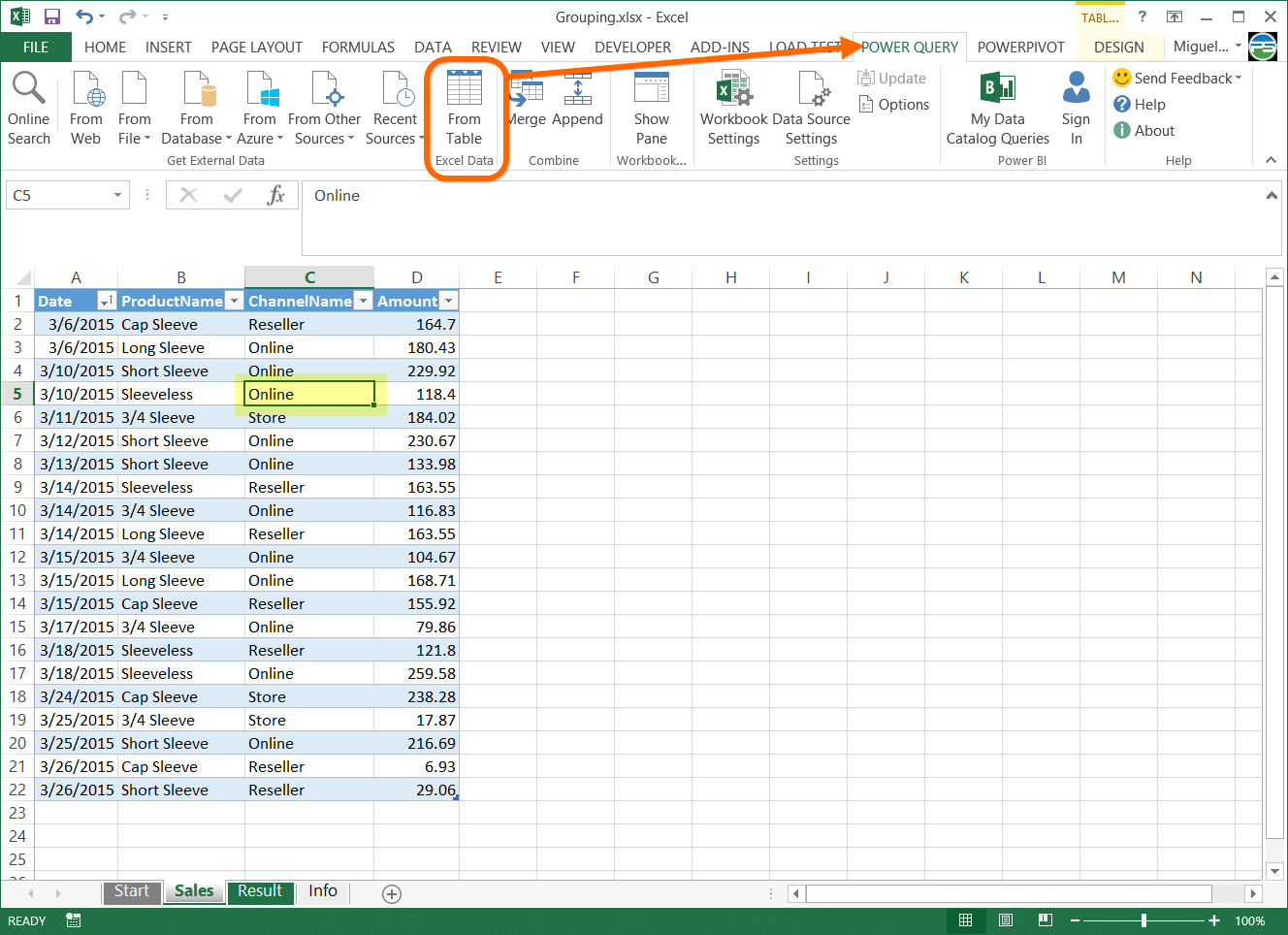
Imagine you have a workbook with a worksheet called Sales, where you’ll find a table. Select any cell inside that table, click the Power Query tab and choose From Table.
You’ll now be launched into the Power Query editor.
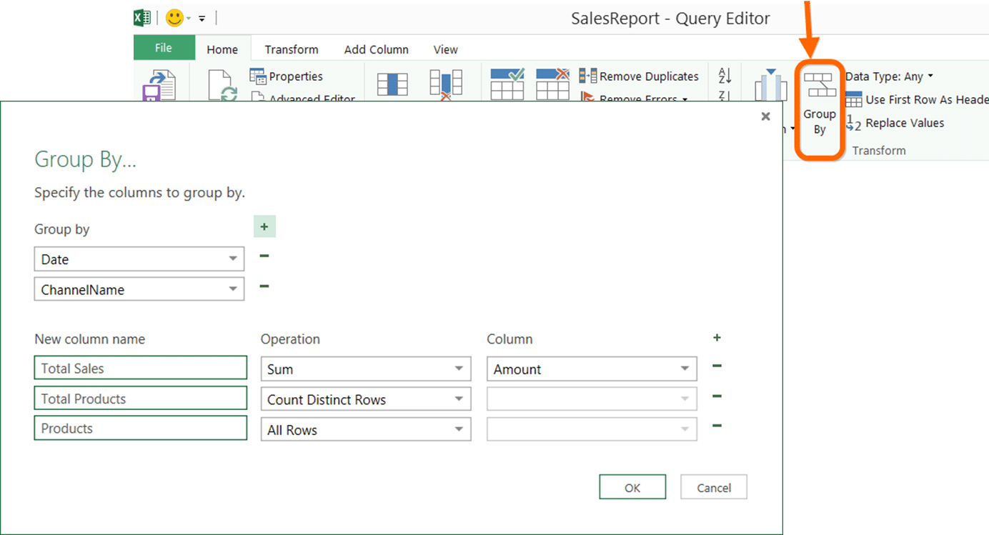
Our first step starts by grouping the rows in our table using some criteria. Click the Group By button and set it up using the following criteria:
That should give us a table with a fewer amount of rows because all the data has been grouped by Date and Channel Name. We’ve even managed to create some new data as well, by creating a SUM of the Amount column, and a Count of Distinct Rows (yielding a count of distinct products by channel by day). We’ve also got a list of all products in the final step, which will make a bit more sense later…
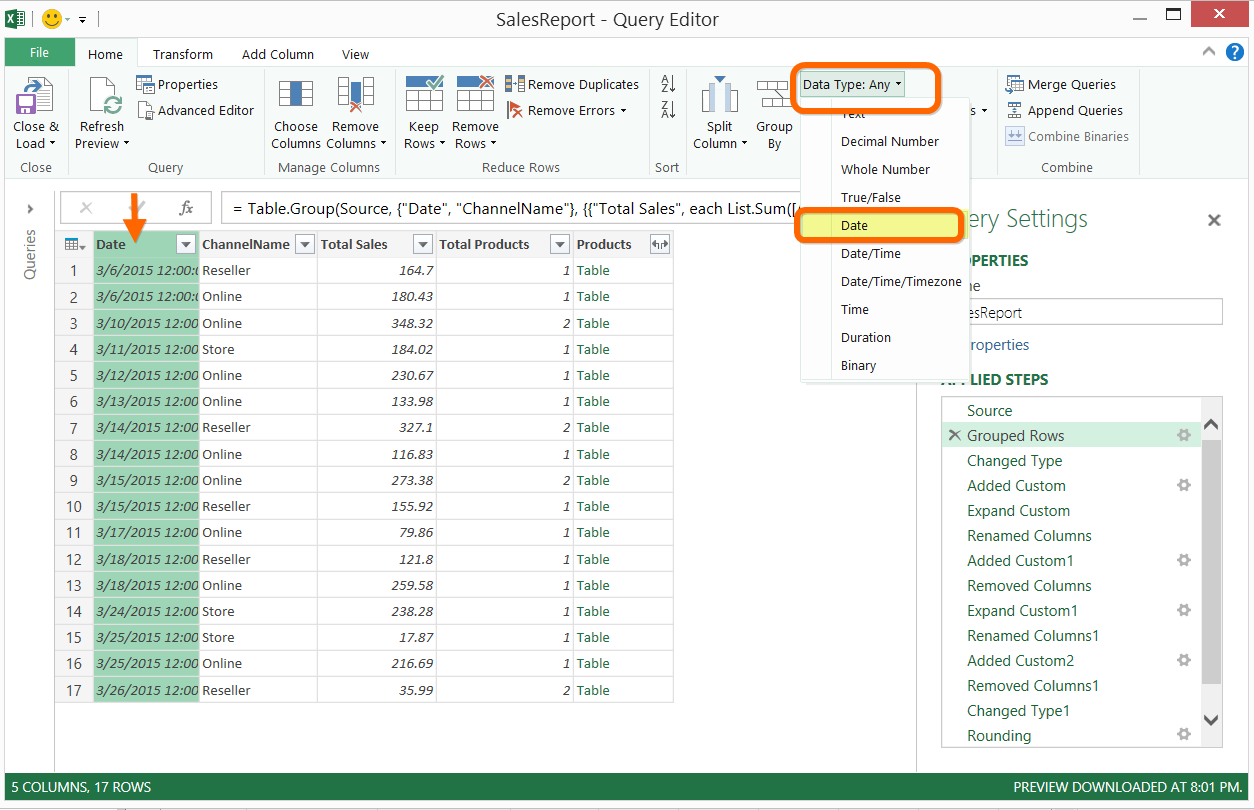
Whenever you pull a date into Power Query, we highly recommend that you specifically define the datatype for the date column. If you don’t, the data could be treated as type “any”, which means that it could land as either text or a value in your output instead of a date. It’s not hard to do at all, simply select the column header, go to the Transform tab, and change the Data Type to Date:
So we’ve now got a Total Sales and a Total Products by Channel, finishing our first goal.
Our next step is to create a formula for a new column that somehow:
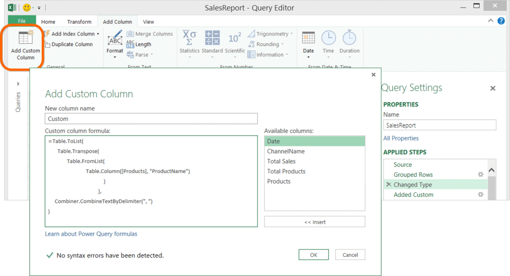
This is the formula that does just that using Table.ToList Table.Transpose Table.FromList Table.Column and the Combiner function:
Table.ToList( Table.Transpose(
 Table.FromList(
 Table.Column([Products], "ProductName")
 )
 ),
 Combiner.CombineTextByDelimiter(", ")
 )
What this formula is doing?
To better explain what this formula is doing, we are going to do each part of that formula as a new step. The formula defined above basically does all of these steps in a single step.
We start with the most inner function and that is Table.Column([Products], “ProductName”):
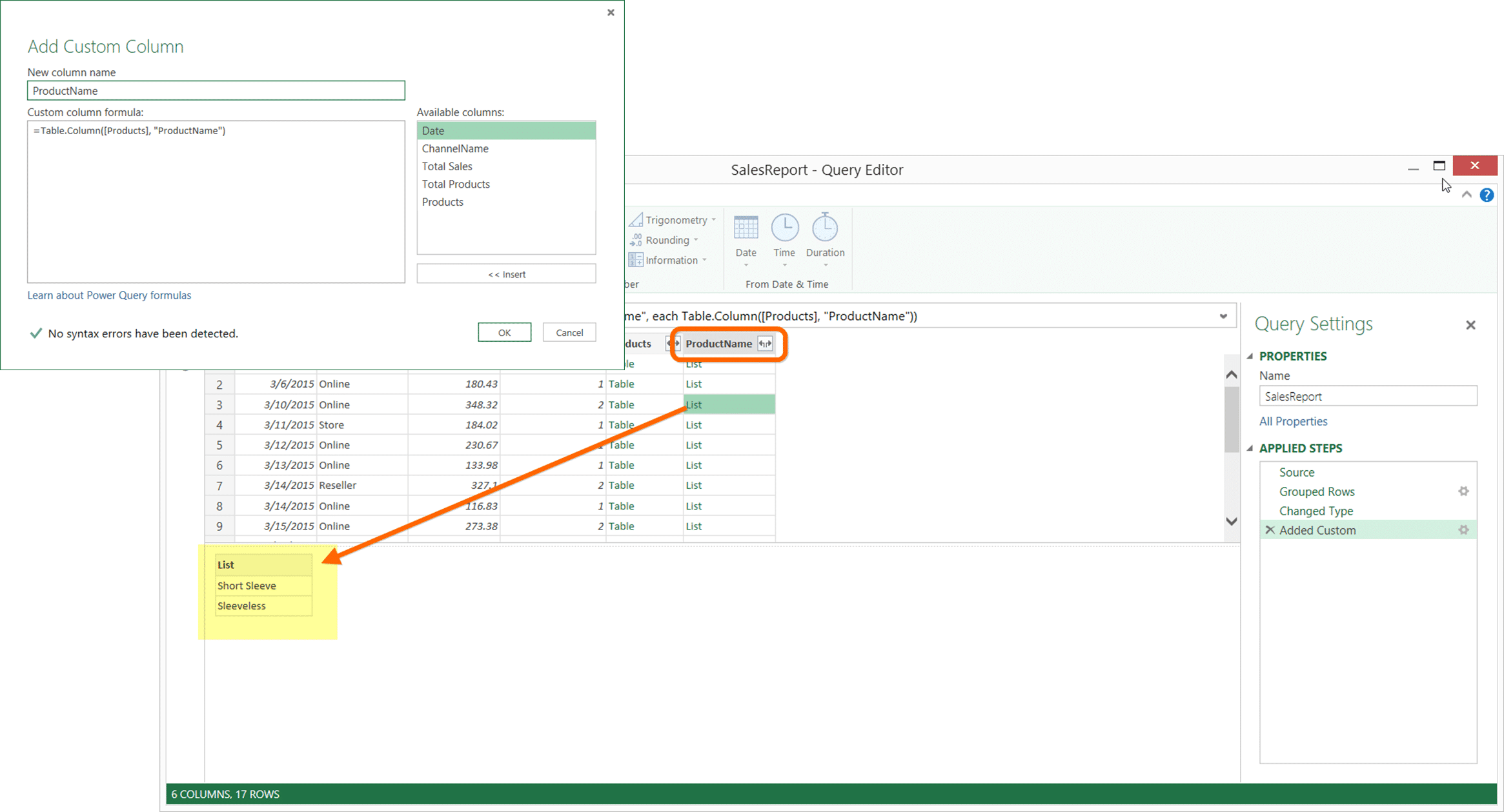
What this formula does is simply extract a column from a table and present it to us a List. So we end up having a list with the values from the ProductName column.
The next step is to transform that list into a Table so it can be easier for us to perform other type of operations. The function that transform a list into a table is called Table.FromList and we’ll use it now:
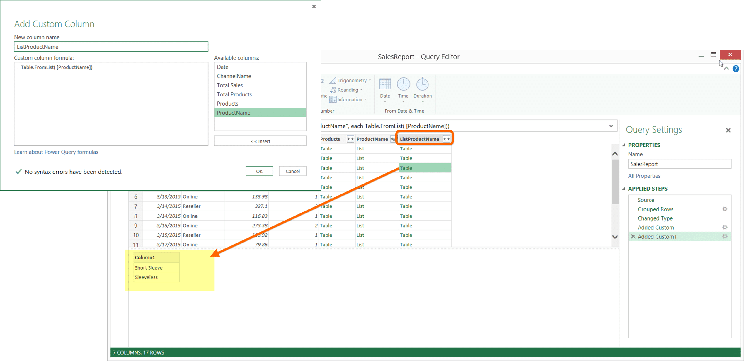
As you can see from the picture above, the new column has Table values for that whole column. We did that because we want to use another function to transpose those rows into columns. That function is Table.Transpose and that formula should read like this:
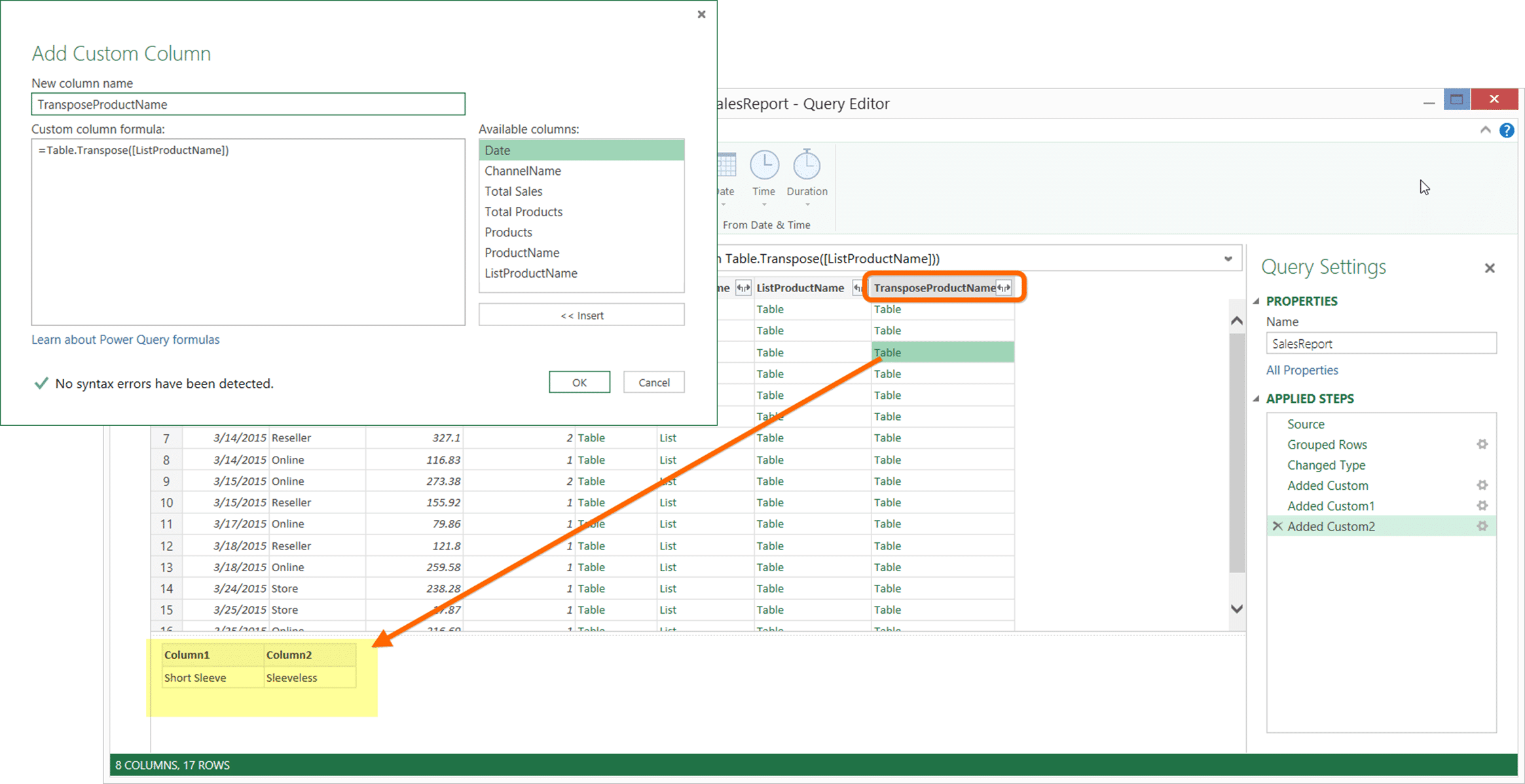
The result of that is basically a transposed table. So if we had N amount of rows and only 1 column now we’ll have 1 row with N amount of columns.
Our next step is to combine all the columns using a format similar to “Value1, Value2, Value3, …, ValueN”.
To do that, we use a Table.ToList that automatically does the operation of concatenating all of the strings into a single value. By Default, it uses a comma separator but in this case we want to go with a comma followed by a space (, ) and the second argument of Table.ToList allow us to do so by adding a Combiner function.
In our case, we’ll use this combiner function: Combiner.CombineTextByDelimiter(“, “) that does just exactly what we need.
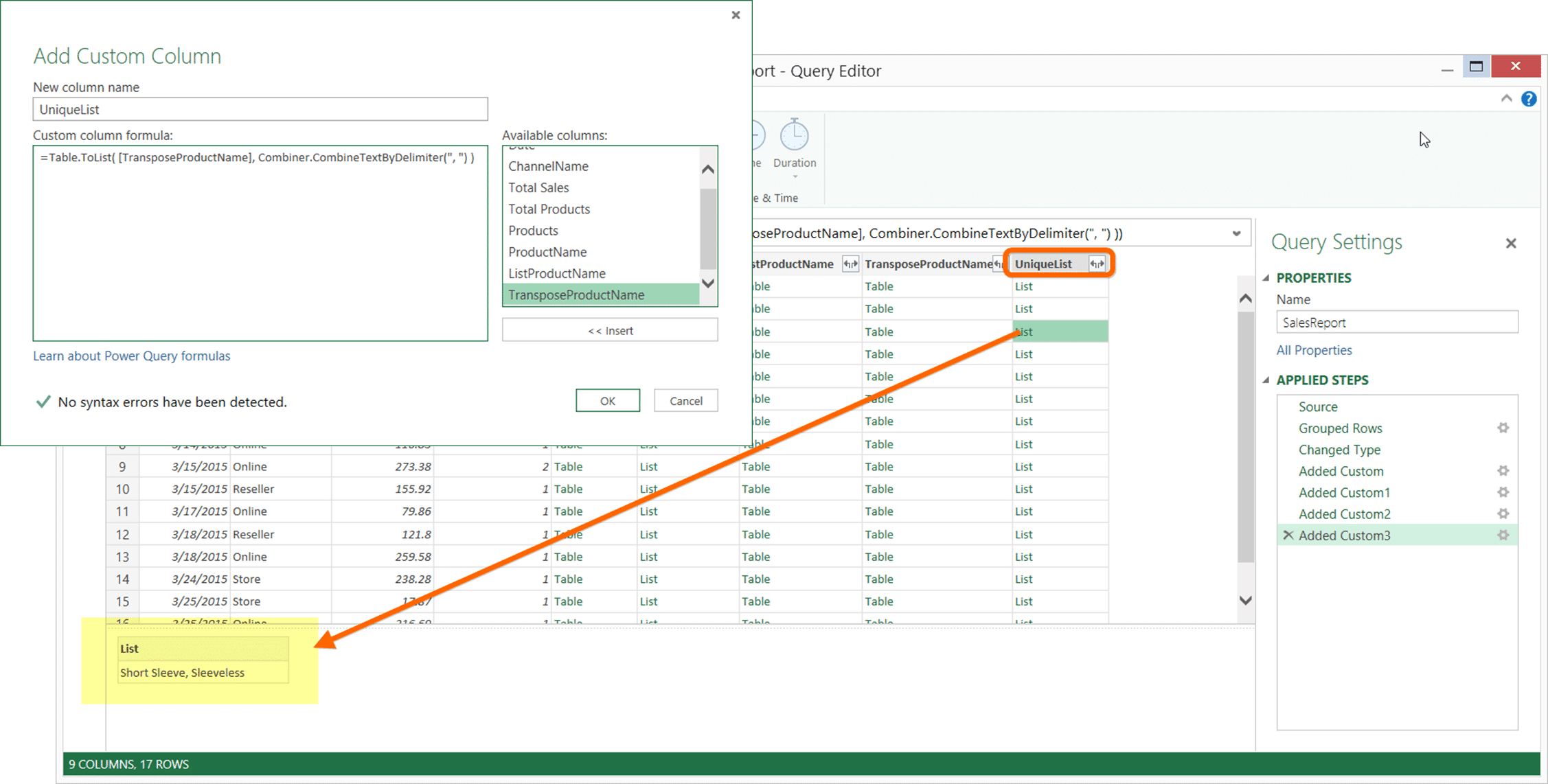
And once you expand that column by clicking the arrows that go in opposite directions, and once we rename that column, this is the result of it:
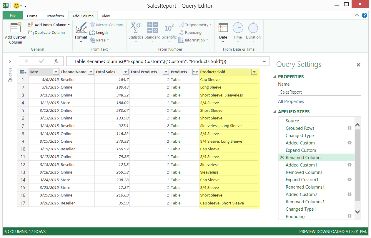
We created the column that creates the list of all the products that were sold on that day, so we finished our 2nd goal. Let’s go to the next one.
Our next step is to extract the top product and also its amount on a row by row basis from the column Products which is this case is a table. We can do so by using a new custom column with the following Table.Max function:
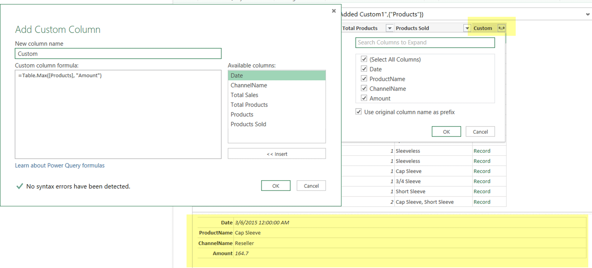
Once you create this new column, you’ll notice that it’ll populate with records which is a special type of data representation in Power Query and what we need is to extract the ProductName and Amount from that record.
We can do so by simply clicking on the opposite arrows icon that are next to the name of this new column. Click on that icon and you’ll notice a new selection window where you can select what columns you want to extract from that record. For now, just select the ProductName and the Amount columns.
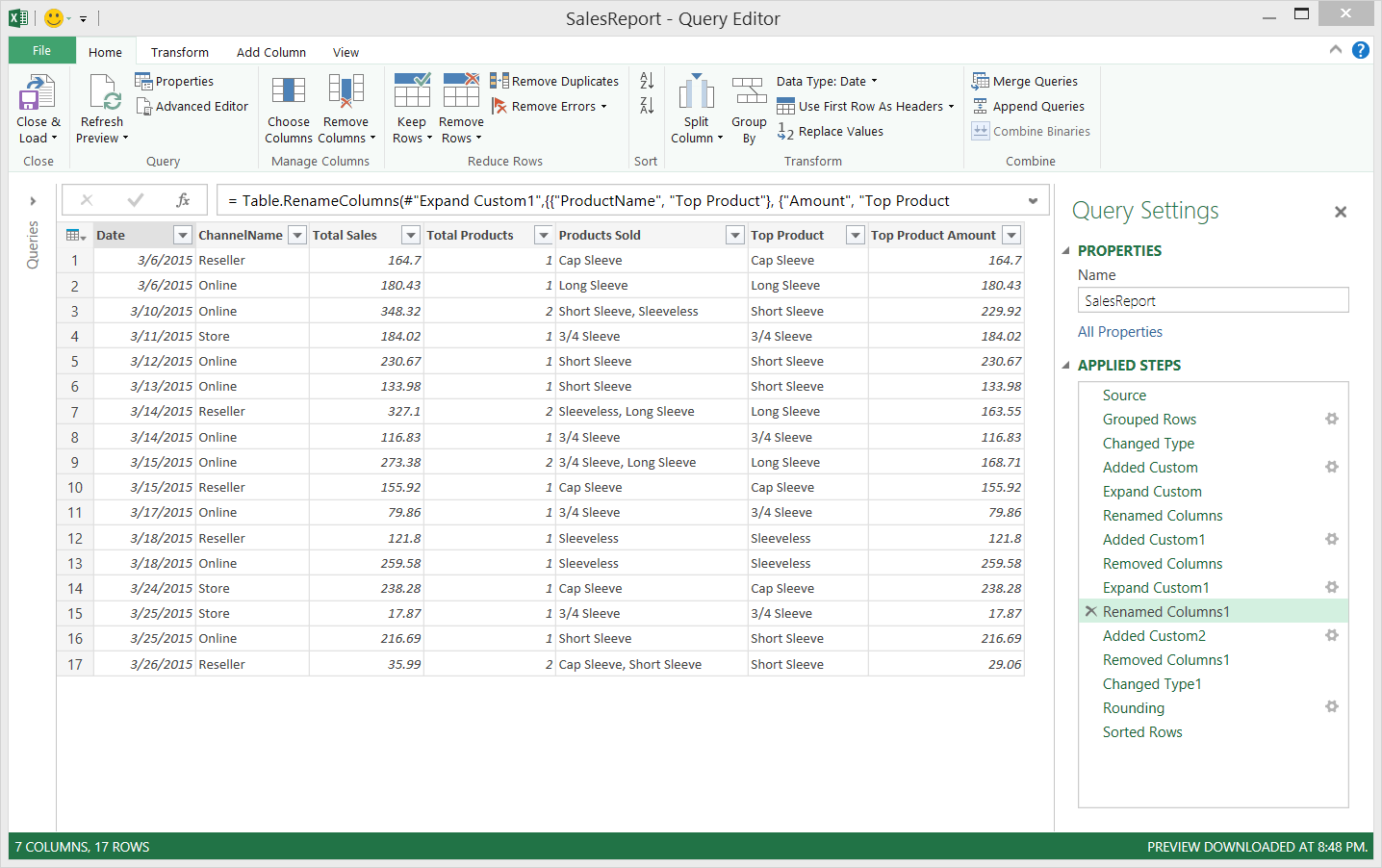
Once we rename those columns this is how our table should look like:
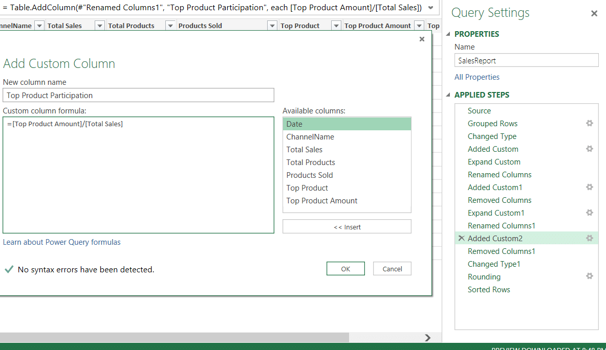
We are almost there! we are missing the division of the Top Product amount over the Total Sales so we can get a % out of it. Let’s do so by adding a new custom column:
After spending some more time cleaning the data, this should be the result of our hard work:
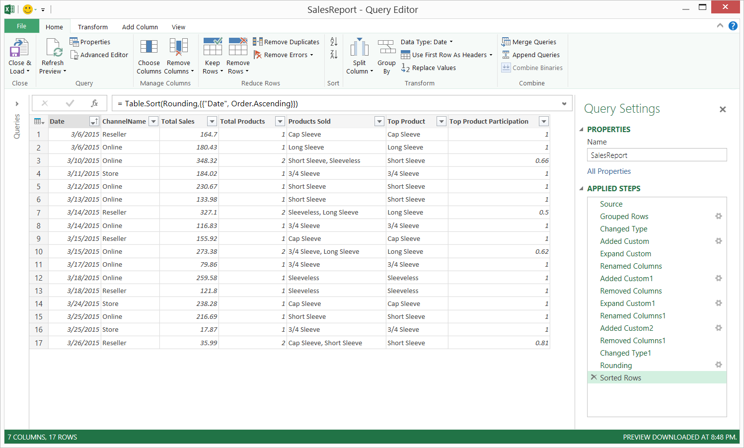
You can click on Close & Load to save this table to your Workbook or inside your Data Model.
Note that you can refresh this at any time and it’ll work as desired.
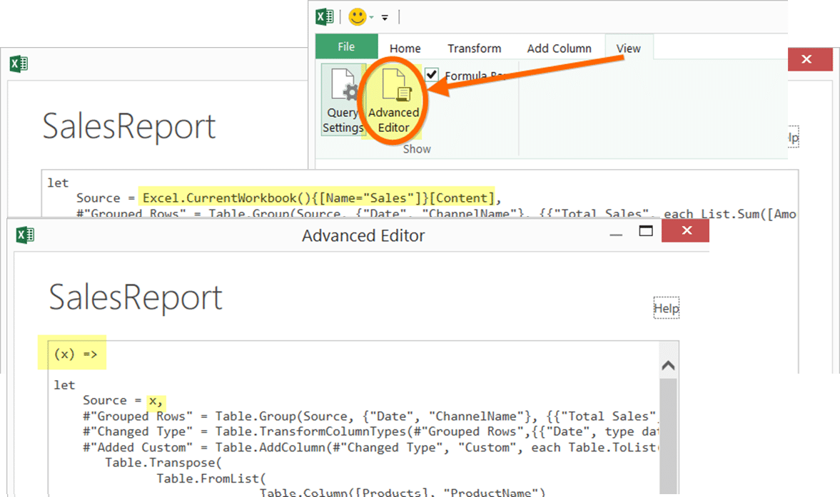
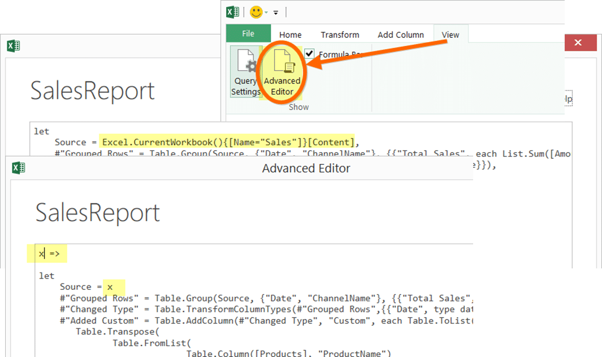
There are many ways to transform this into a function, but the basics of creating a function go into making a part of the whole code a variable.
Which one would you choose to make a variable? Let us know in the comments section below
This time, we’re choosing a simple variable. Since we need the Source step to be a table, let’s define that as our variable.
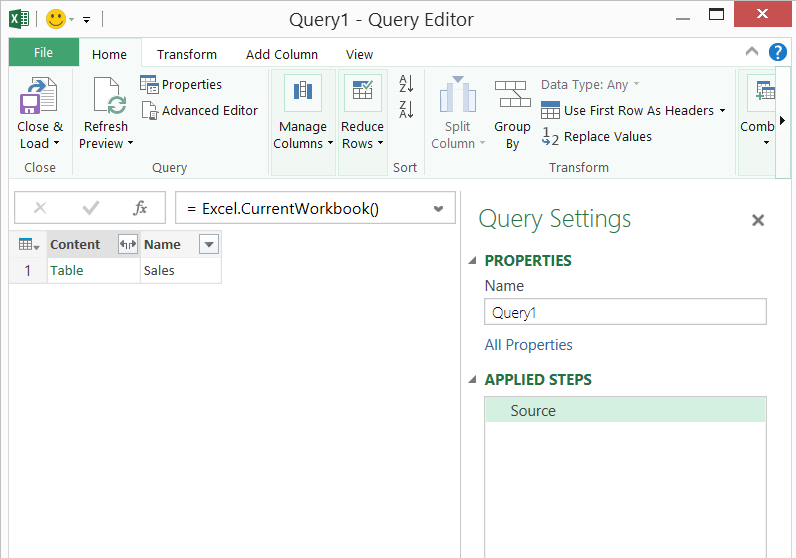
Now we need to put this to the test. Let’s create a blank query and grab all the tables from our current Workbook using Excel.CurrentWorkbook():
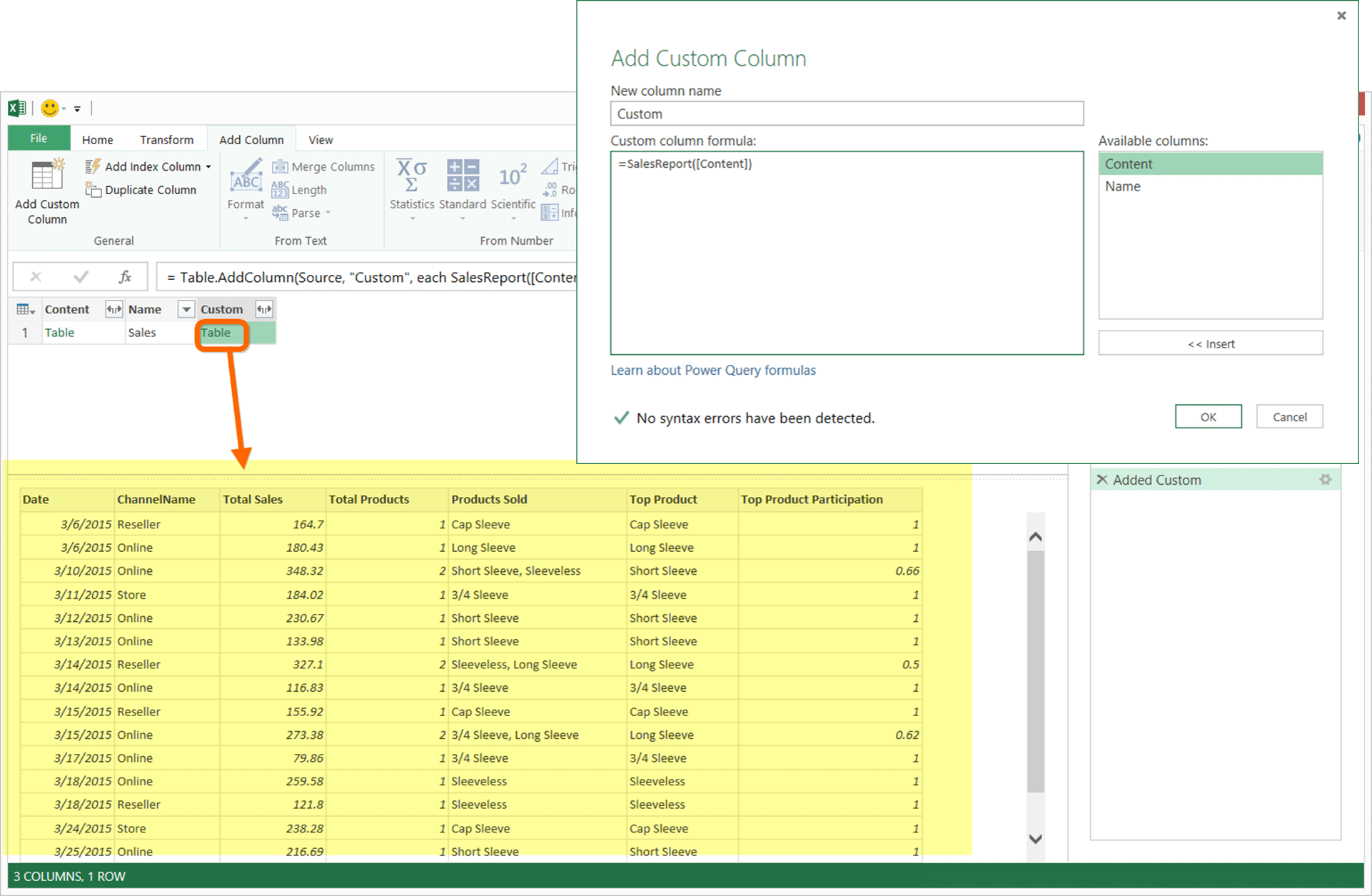
Next we add a custom column by using the name of the function that we just created which is the name of the Query SalesReport and the result should look like this: